Chapter 2 Data Processing

1. Prepare data tables (minimum: count matrix, column data)
2. Compile all data into an .RData or .db object.

---

2.1 Preparation

To implement this app, you will need three types of data:

1. Count tables in ./data/CountTables/ folder
   

• This contains the count matrix
  
• The first column of count matrix must gene symbols
  
• The column names of your count table must be the same as the rownames of your ‘colData’ (see below).

X	Sample50_BALB.c_SHAM_M	Sample51_BALB.c_SHAM_M	Sample55_BALB.c_SHAM_F	Sample56_BALB.c_SHAM_F	Sample57_BALB.c_SHAM_F	Sample58_B10.D2_SHAM_M	Sample60_B10.D2_SHAM_M	Sample67_B10.D2_SHAM_F	Sample71_BALB.c_SHAM_M	Sample77_B10.D2_SHAM_F	Sample88_B10.D2_SHAM_M	Sample49_BALB.c_SNI_M	Sample64_BALB.c_SNI_F	Sample65_BALB.c_SNI_F	Sample69_B10.D2_SNI_F	Sample70_BALB.c_SNI_M	Sample76_B10.D2_SNI_F	Sample78_B10.D2_SNI_F	Sample89_B10.D2_SNI_M	Sample90_B10.D2_SNI_M	symbol
ENSMUSG00000000001	20.6460082	20.9684737	25.6051105	17.9245459	21.8279448	23.8898091	20.8612482	21.1079774	21.9353412	19.8810344	25.4903826	23.2414339	26.0955758	24.5983920	22.3698430	25.4514816	23.2571636	25.0393354	21.4696758	21.4316521	Gnai3
ENSMUSG00000000003	0.0000000	0.0000000	0.0000000	0.0000000	0.0000000	0.0000000	0.0000000	0.0000000	0.0000000	0.0000000	0.0000000	0.0000000	0.0000000	0.0000000	0.0000000	0.0000000	0.0000000	0.0000000	0.0000000	0.0000000	Pbsn
ENSMUSG00000000028	1.2444692	1.0386601	1.4225152	0.8771354	0.7774382	0.9572740	0.6793672	0.8532159	0.9904448	0.8884526	1.1943520	1.4496099	1.0502148	0.9892706	0.8066116	0.8839994	0.9460189	0.9714055	0.9352520	0.9411879	Cdc45
ENSMUSG00000000031	146.6304065	78.6870749	279.4541932	122.2226711	86.5995137	385.7192026	402.3015644	373.7624763	83.4889245	416.2586323	523.7706518	34.6120591	215.3297763	259.9150108	642.1622405	103.1170442	510.7111982	497.6381737	213.8979427	462.2669044	H19
ENSMUSG00000000037	0.0673974	0.0434038	0.0736720	0.0567710	0.0603054	0.0782123	0.0638765	0.0663909	0.0661561	0.0811122	0.1074937	0.0509788	0.0717639	0.0585030	0.0728068	0.0970444	0.0831925	0.1111677	0.0729349	0.0880621	Scml2
ENSMUSG00000000049	0.0895870	0.0961564	0.0699482	0.0611854	0.1214547	0.1831722	0.1309992	0.1764983	0.0713003	0.1952917	0.2609194	0.1016442	0.0931727	0.0818572	0.1539641	0.1098845	0.2628942	0.1581742	0.1856444	0.2387010	Apoh

 

2. Column Data (abbrev: colData) in ./data/ColDatas/ folder
   

• This contains the info about each sample
  
• The rownames of ‘colData’ must be the same as the column names of your count table.
• The colnames of colData must include ‘Condition’, which specifies the disease/healthy condition of your samples.
  
• If your experiment contains additional parameters such as Population, Timepoint, and Sex, you will need to rename them to this format.

	X	Sample	Population	Condition	Sex	Sample_Pop_Cond_Sex	Dataset	Species	Timepoint
Sample50_BALB.c_SHAM_M	Sample50_BALB.c_SHAM_M	Sample50	BALB.c	SHAM	M	Sample50_BALB.c_SHAM_M	Bulk DRG	Mouse (DRG)	na
Sample51_BALB.c_SHAM_M	Sample51_BALB.c_SHAM_M	Sample51	BALB.c	SHAM	M	Sample51_BALB.c_SHAM_M	Bulk DRG	Mouse (DRG)	na
Sample55_BALB.c_SHAM_F	Sample55_BALB.c_SHAM_F	Sample55	BALB.c	SHAM	F	Sample55_BALB.c_SHAM_F	Bulk DRG	Mouse (DRG)	na
Sample56_BALB.c_SHAM_F	Sample56_BALB.c_SHAM_F	Sample56	BALB.c	SHAM	F	Sample56_BALB.c_SHAM_F	Bulk DRG	Mouse (DRG)	na
Sample57_BALB.c_SHAM_F	Sample57_BALB.c_SHAM_F	Sample57	BALB.c	SHAM	F	Sample57_BALB.c_SHAM_F	Bulk DRG	Mouse (DRG)	na
Sample58_B10.D2_SHAM_M	Sample58_B10.D2_SHAM_M	Sample58	B10.D2	SHAM	M	Sample58_B10.D2_SHAM_M	Bulk DRG	Mouse (DRG)	na

 

3. Differential expression data frames (abbrev: deg_df) in ./data/DegData/ folder
   

• This data file contains the log2FoldChange and statistics of one case vs control
• An experiment can have multiple deg_df files

	baseMean	log2FoldChange	lfcSE	stat	pvalue	padj	symbol	Population
ENSMUSG00000109908	10.737773	6.453185	4.103313	1.572677	NA	NA	NA	b10d2
ENSMUSG00000096108	4.372395	-6.405612	3.800576	-1.685432	0.0919053	NA	NA	b10d2
ENSMUSG00000095889	3.541538	-6.168911	4.228860	-1.458765	0.1446299	NA	NA	b10d2
ENSMUSG00000073494	5.130631	5.941862	1.068377	5.561578	0.0000000	NA	Sh2d1b2	b10d2
ENSMUSG00000036357	3.708027	5.483357	1.130411	4.850764	0.0000012	NA	Gpr101	b10d2
ENSMUSG00000076538	3.050185	-5.384935	1.643832	-3.275843	0.0010535	NA	NA	b10d2

2.2 Species (optional)

If your data contains different species, you will also need datasets that allow you map gene symbols/IDs between species. We have provided an option using the biomaRt library.

library("biomaRt")
mouse = useMart("ensembl", dataset = "mmusculus_gene_ensembl", verbose = TRUE, host = "https://dec2021.archive.ensembl.org")
human = useMart("ensembl", dataset = "hsapiens_gene_ensembl", verbose = TRUE, host = "https://dec2021.archive.ensembl.org")

human_gene_data = getLDS(attributes = c("mgi_symbol","ensembl_gene_id"), 
                filters = "ensembl_gene_id", 
                values = count$X, 
                mart = mouse, 
                attributesL = c("hgnc_symbol", "ensembl_gene_id", "description"), 
                martL = human, 
                uniqueRows=T)

colnames(human_gene_data) = c("mgi_symbol", "mouse_gene_id", "hgnc_symbol", "human_gene_id")

mgi_symbol	mouse_gene_id	hgnc_symbol	human_gene_id	NA
mt-Nd2	ENSMUSG00000064345	MT-ND2	ENSG00000198763	mitochondrially encoded NADH:ubiquinone oxidoreductase core subunit 2 [Source:HGNC Symbol;Acc:HGNC:7456]
mt-Atp6	ENSMUSG00000064357	MT-ATP6	ENSG00000198899	mitochondrially encoded ATP synthase membrane subunit 6 [Source:HGNC Symbol;Acc:HGNC:7414]
mt-Co2	ENSMUSG00000064354	MT-CO2	ENSG00000198712	mitochondrially encoded cytochrome c oxidase II [Source:HGNC Symbol;Acc:HGNC:7421]
mt-Nd4l	ENSMUSG00000065947	MT-ND4L	ENSG00000212907	mitochondrially encoded NADH:ubiquinone oxidoreductase core subunit 4L [Source:HGNC Symbol;Acc:HGNC:7460]
mt-Co1	ENSMUSG00000064351	MT-CO1	ENSG00000198804	mitochondrially encoded cytochrome c oxidase I [Source:HGNC Symbol;Acc:HGNC:7419]
mt-Nd5	ENSMUSG00000064367	MT-ND5	ENSG00000198786	mitochondrially encoded NADH:ubiquinone oxidoreductase core subunit 5 [Source:HGNC Symbol;Acc:HGNC:7461]

2.3 RData (option 1)

If your experimental data contains managable number of files, you can read them one by one and store them into a list. Name each dataframe object with the name that you will use later.

You can then store the list of dataframes into .RData using the save() function. For example, we can read the the count data frame to list called “mat” and then use the save() function to save it into a file called my_data.RData.

Read count data

mat = list()

# read count data csv into a dataframe 
count = read.csv("./data/CountTables/TPM_mouse.csv", header = TRUE)

# store into 'mat', name the dataframe for accessing it later
mat = append(mat, list("TPM_mouse" = count))

save(mat, file = "my_data.RData")

Read colData, remember to set the rownames to the colnames of your count table

# read count data csv into a dataframe 
colData = read.csv("./data/colData/TPM_mouse_colData.csv", header = TRUE)

# set the rownames 
rownames(colData) = colData[,1]

# store into 'mat', name the dataframe for accessing it later 
mat = append(mat, list("TPM_mouse_colData" = colData))

Process and read differential expression data: If you have multiple DE data, you will need to combine them and add an additional column called ‘Population’.

# read all DE data 
b10d2 = read.csv("./data/DegData/b10d2.csv", header = TRUE)
balb = read.csv("./data/DegData/balb.csv", header = TRUE)

# add 'Population column' 
b10d2$Population = rep("b10d2", nrow(b10d2))
balb$Population = rep("balb", nrow(balb))

# combine them 
deg_df = rbind(b10d2, balb)

# store into 'mat', name the dataframe for accessing it later 
mat = append(mat, list("mouse_deg_df" = deg_df))

To load the data frame from the .RData file later, you can use the load() function in your server.

load("my_data.RData") # add to server

# you can then access the dataframe using its name 
df = mat[["TPM_mouse"]]

NOTE, some functions will need to be modified to read from a .RData instead. This can be done by uncommentng the relevant lines of code. For example:

  shiny::observeEvent(input$load, {
    
    if (include_count == TRUE){
      # query count datasets
      
      ## comment here for .RData file
      # for database 
      {
        if (species == "human") {
          sql = paste("SELECT * FROM", count_df, "WHERE mgi_symbol = ?")
        }
        else{
          sql = paste("SELECT * FROM", count_df, "WHERE symbol = ?")
        }
        filt = RSQLite::dbGetPreparedQuery(conn, sql, bind.data=data.frame(symbol=genes()))
        filt = as.data.frame(filt)
      }
      
      ## uncomment here for .RData file
      # using R Data 
      {
        # count_df = mat[["count_df"]]
        # if (species == "human"){
        #   filt = count_df[count_df$mgi_symbol %in% genes(),]
        #   X = rownames(filt)
        #   filt = cbind(X, filt)
        #   
        # }
        # else {
        #   filt = count_df[count_df$symbol %in% genes(),]
        #   X = rownames(filt)
        #   filt = cbind(X, filt)
        # }
      }

If you plan to store data this way, move to the User Interface section now. If you are working with larger amounts of data, you may find it useful to set up an SQL database (recommended, below).

2.4 Building an SQL database via R (recommended)

While .RData files can be useful small or medium-sized datasets in R, SQL databases provide a more powerful and flexible solution for managing large, complex datasets that need to be shared, queried, and analyzed by multiple users or integrated with other tools and applications.

An SQLite database consists of one or more tables, which are composed of rows and columns. An RSQLite .db object is a database connection to a SQLite database file through R. The following functions will be useful in creating and updating the .db object in R.

Here, we provide an overview for bulk count data. Seurat objects (for sc/snRNA-seq or ATAC-seq) are read in separately.

# This function connects to a SQLite database file called `example_database.db`
db_dir = "example_database.db" 
conn  <- dbConnect(RSQLite::SQLite(), db_dir)

# This function stores dataframe objects into `.db` object 
dbWriteTable(conn, name = "count_df", value = count, row.names = TRUE, append=TRUE)

2.4.1 SQL manipulation

# List table names that you have already stored  
dbListTables(conn)

# Modify a table by using 'overwrite' argument 
dbWriteTable(conn, name = "count_df", value = count_modified, overwrite = TRUE)

Each table in a SQLite database has a schema that defines the columns in the table and their data types. In R, you can retrieve the schema of a table using the dbListFields() function, which returns a character vector of the column names.

# Get the schema of the "count_df" table
fields <- dbListFields(conn, "count_df")

The dbGetQuery() function in RSQLite allows you to execute SQL queries and return the results as a data frame.

# Select all rows from the "count_df" table
result <- dbGetQuery(conn, "SELECT * FROM count_df")

# Delete a table 
dbRemoveTable(conn, "count_df")

# Close the connection after you stored all tables
dbDisconnect(conn)

These functions are sufficient for users without prior knowledge in the RSQLite package. Further tutorials can be found at https://www.datacamp.com/tutorial/sqlite-in-r

2.4.2 Processing multiple files

If your experimental data contains multiple files, it can become labor intensive to write tables one by one. To reduce the burden, you can read files by folders.

Read all count tables in ./data/CountTables folder into .db object, using their file names as table names.

# all file names 
Counts <- str_sort(list.files(path = "./data/CountTables", pattern = "*.csv")) # names of the count tables

# name each file as their file name without ".csv" suffix 
names = as.vector(substr(Counts, 0, nchar(Counts) - 4))

# read files into database, using their file names as table names 
for (i in 1:length(names)){
  name  = names[i]
  value = read.csv(paste0("./data/CountTables/", Counts[i]), header = TRUE)
  dbWriteTable(conn, name, value, row.names = TRUE)
}

Read ColDatas files in ./data/ColDatas directory into tables.
NOTE you must set and read in the row names of colData

CDs <- str_sort(list.files(path = "./data/ColDatas", pattern = "*.csv")) # names of colDatas 

names <- substr(CDs, 0, nchar(CDs) - 4)# assign name 

# read in colData
for (i in 1:length(names)) {
  name  = names[i]
  value = read.csv(paste0("./data/ColDatas/", CDs[i]), header = TRUE, row.names = 1)
  dbWriteTable(conn, name, value, row.names = TRUE, overwrite = TRUE)
}

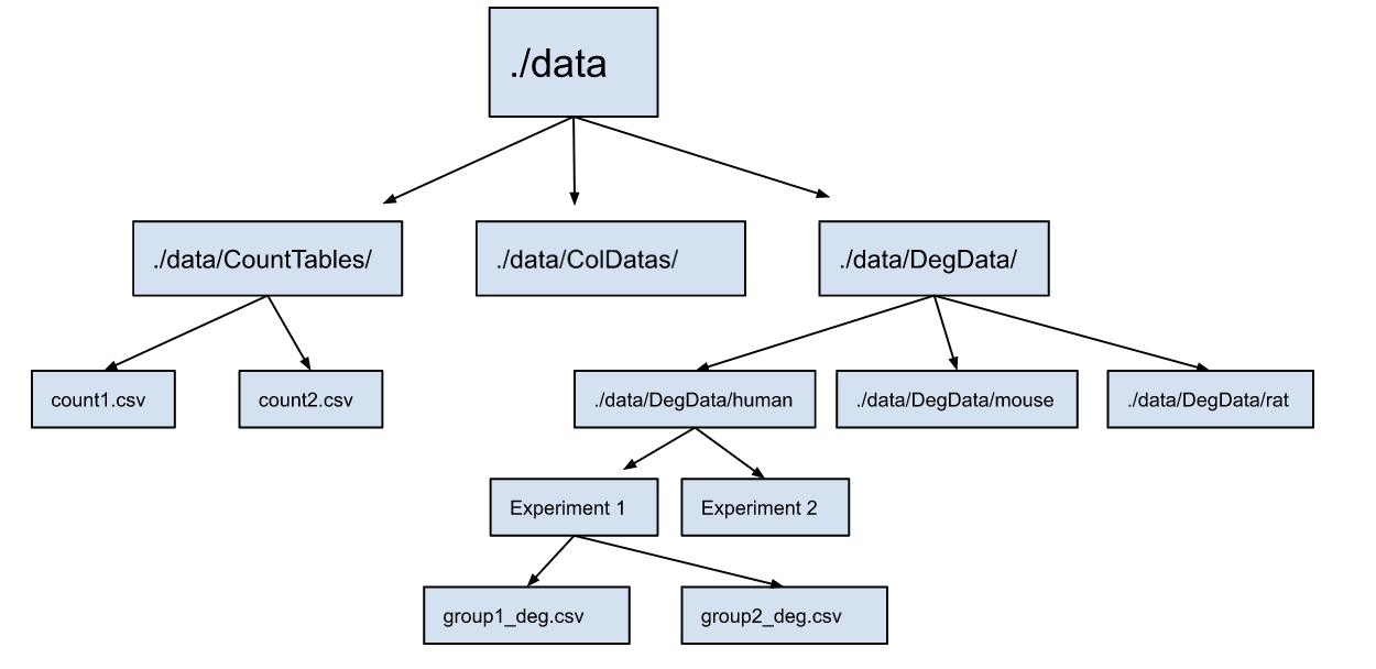
Reading in differential expression files in ./data/DegData/ directory: You can store them into different sub-directories based on species, as illustrated here. A combined deg_df for each species is generated and stored, which makes meta-analysis and cross-species comparison easier.

In addition, since some experiments contain more than one differential expression analysis file, they are combined into one for each experiment, as illustrated below. To do this, you will need to store multiples into a folder for each study. A schematic illustration is shown below:

# table names for files 
## assign names here
deg_df_names = c("subtype_deg_df", "mouse_deg_df", "rat_deg_df", "ipsc_deg_df", "db_deg_df", "cts_deg_df")

# you need to specify the names of the dataset (experiments) and store them in the list below
## assign names here
Dataset = c("mouse/Subtype DRG (Barry)/", "mouse/Mouse DRG Bulk/", "rat/Rat DRG Bulk/",
            "human/Human iPSC HSN1/", "human/Human skin Diabetes/", "human/Human skin Carpal Tunnel (CTS)/")

## just run this
human_deg_df = data.frame()
mouse_deg_df = data.frame()
rat_deg_df   = data.frame()

# for each experiment
for (j in 1:length(Dataset)) {
  
  # name of experiment
  name = Dataset[j] 
  
  # species  
  species = unlist(strsplit(name, split = "/"))[[1]]
  
  # DEs are a list of datasets in this experiment 
  DEs = str_sort(list.files(path = paste("./data/DegData/", name, sep=""), pattern = "*.csv"))
  DE_names <- substr(DEs, 0, nchar(DEs) - 4)# assign name to each population
  deg_list = list()
  
  # read in those datasets into one dataframes for each experiment
  for (i in 1:length(DE_names)) {
    df_name = DE_names[i]
    value   = read.csv(paste("./data/DegData/", name, DEs[i], sep=""), header = TRUE, row.names = 1)
    deg_list = append(deg_list, list(value))
  }
  
  dataset_combine_deg = generate_degdf(deg_list, DE_names, unlist(strsplit(name, split = "/"))[[2]])
  dbWriteTable(conn, deg_df_names[j], dataset_combine_deg)
  
  # add to species-specific lists of data frames 
  if (species == "human"){
    human_deg_df = rbind(human_deg_df, dataset_combine_deg)
  }
  if (species == "mouse"){
    mouse_deg_df = rbind(mouse_deg_df, dataset_combine_deg)
  }
  if (species == "rat"){
    rat_deg_df = rbind(rat_deg_df, dataset_combine_deg)
  }
  
}

# write species deg_df into table
dbWriteTable(conn, "mouse_all_deg_df", mouse_deg_df)
dbWriteTable(conn, "human_deg_df", human_deg_df)
dbWriteTable(conn, "rat_deg_df", rat_deg_df)

Now, the .db object should contain all data required to run your app.